2.2. Tricks for Training
2.2.1. Choice of Optimizers:
Since the development of deep learning, there have been many researchers working on the optimizer. The purpose of the optimizer is to make the loss function as small as possible, so as to find suitable parameters to complete a certain task. At present, the main optimizers used in model training are SGD, RMSProp, Adam, AdaDelt and so on. The SGD optimizers with momentum is widely used in academia and industry, so most of models we release are trained by SGD optimizer with momentum. But the SGD optimizer with momentum has two disadvantages, one is that the convergence speed is slow, the other is that the initial learning rate is difficult to set, however, if the initial learning rate is set properly and the models are trained in sufficient iterations, the models trained by SGD with momentum can reach higher accuracy compared with the models trained by other optimizers. Some other optimizers with adaptive learning rate such as Adam, RMSProp and so on tent to converge faster, but the final convergence accuracy will be slightly worse. If you want to train a model in faster convergence speed, we recommend you use the optimizers with adaptive learning rate, but if you want to train a model with higher accuracy, we recommend you to use SGD optimizer with momentum.
2.2.2. Choice of Learning Rate and Learning Rate Declining Strategy:
The choice of learning rate is related to the optimizer, data set and tasks. Here we mainly introduce the learning rate of training ImageNet-1K with momentum + SGD as the optimizer and the choice of learning rate decline.
2.2.2.1. Concept of Learning Rate:
the learning rate is the hyperparameter to control the learning speed, the lower the learning rate, the slower the change of the loss value, though using a low learning rate can ensure that you will not miss any local minimum, but it also means that the convergence speed is slow, especially when the gradient is trapped in a gradient plateau area.
2.2.2.2. Learning Rate Decline Strategy:
During training, if we always use the same learning rate, we cannot get the model with highest accuracy, so the learning rate should be adjust during training. In the early stage of training, the weights are in a random initialization state and the gradients are tended to descent, so we can set a relatively large learning rate for faster convergence. In the late stage of training, the weights are close to the optimal values, the optimal value cannot be reached by a relatively large learning rate, so a relatively smaller learning rate should be used. During training, many researchers use the piecewise_decay learning rate reduction strategy, which is a stepwise decline learning rate. For example, in the training of ResNet50, the initial learning rate we set is 0.1, and the learning rate drops to 1/10 every 30 epoches, the total epoches for training is 120. Besides the piecewise_decay, many researchers also proposed other ways to decrease the learning rate, such as polynomial_decay, exponential_decay and cosine_decay and so on, among them, cosine_decay has become the preferred learning rate reduction method for improving model accuracy beacause there is no need to adjust hyperparameters and the robustness is relatively high. The learning rate curves of cosine_decay and piecewise_decay are shown in the following figures, it is easy to observe that during the entire training process, cosine_decay keeps a relatively large learning rate, so its convergence is slower, but the final convergence accuracy is better than the one using piecewise_decay.
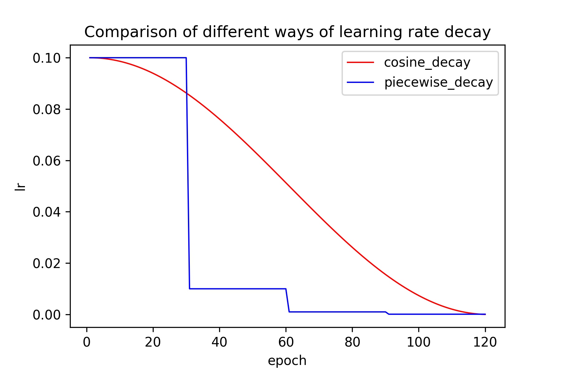
In addition, we can also see from the figures that the number of epoches with a small learning rate in cosine_decay is fewer, which will affect the final accuracy, so in order to make cosine_decay play a better effect, it is recommended to use cosine_decay in large epoched, such as 200 epoches.
2.2.2.3. Warmup Strategy
If a large batch_size is adopted to train nerual network, we recommend you to adopt warmup strategy. as the name suggests, the warmup strategy is to let model learning first warm up, we do not directly use the initial learning rate at the begining of training, instead, we use a gradually increasing learning rate to train the model, when the increasing learning rate reaches the initial learning rate, the learning rate reduction method mentioned in the learning rate reduction strategy is then used to decay the learning rate. Experiments show that when the batch size is large, warmup strategy can improve the accuracy. Some model training with large batch_size such as MobileNetV3 training, we set the epoch in warmup to 5 by default, that is, first in 5 epoches, the learning rate increases from 0 to initial learning rate, then learning rate decay begins.
2.2.3. Choice of Batch_size
Batch_size is an important hyperparameter in training neural networks, batch_size determines how much data is sent to the neural network to for training at a time. In the paper [1], the author found in experiments that when batch_size is linearly related to the learning rate, the convergence accuracy is hardly affected. When training ImageNet data, an initial learning rate of 0.1 are commonly chosen for training, and batch_size is 256, so according to the actual model size and memory, you can set the learning rate to 0.1*k, batch_size to 256*k.
2.2.4. Choice of Weight_decay
Overfitting is a common term in machine learning. A simple understanding is that the model performs well on the training data, but it performs poorly on the test data. In the convolutional neural network, there also exists the problem of overfitting. To avoid overfitting, many regular ways have been proposed. Among them, weight_decay is one of the widely used ways to avoid overfitting. After the final loss function, L2 regularization(weight_decay) is added to the loss function, with the help of L2 regularization, the weight of the network tend to choose a smaller value, and finally the parameters in the entire network tends to 0, and the generalization performance of the model is improved accordingly. In different kinds of Deep learning frame, the meaning of L2_decay is the coefficient of L2 regularization, on paddle, the name of this value is L2_decay, so in the following the value is called L2_decay. the larger the coefficient, the more the model tends to be underfitting. In the task of training ImageNet, this parameter is set to 1e-4 in most network. In some small networks such as MobileNet networks, in order to avoid network underfitting, the value is set to 1e-5 ~ 4e-5. Of course, the setting of this value is also related to the specific data set, When the data set is large, the network itself tends to be under-fitted, and the value can be appropriately reduced. When the data set is small, the network tends to overfit itself, so the value can be increased appropriately. The following table shows the accuracy of MobileNetV1_x0_25 using different l2_decay on ImageNet-1k. Since MobileNetV1_x0_25 is a relatively small network, the large l2_decay will make the network tend to be underfitting, so in this network, 3e-5 are better choices compared with 1e-4.
| Model | L2_decay | Train acc1/acc5 | Test acc1/acc5 |
|---|---|---|---|
| MobileNetV1_x0_25 | 1e-4 | 43.79%/67.61% | 50.41%/74.70% |
| MobileNetV1_x0_25 | 3e-5 | 47.38%/70.83% | 51.45%/75.45% |
In addition, the setting of L2_decay is also related to whether other regularization is used during training. If the data argument during the training is more complicated, which means that the training becomes more difficult, L2_decay can be appropriately reduced. The following table shows that the precision of ResNet50 using a different l2_decay on ImageNet-1K. It is easy to observe that after the training becomes difficult, using a smaller l2_decay helps to improve the accuracy of the model.
| Model | L2_decay | Train acc1/acc5 | Test acc1/acc5 |
|---|---|---|---|
| ResNet50 | 1e-4 | 75.13%/90.42% | 77.65%/93.79% |
| ResNet50 | 7e-5 | 75.56%/90.55% | 78.04%/93.74% |
In summary, l2_decay can be adjusted according to specific tasks and models. Usually simple tasks or larger models are recommended to use Larger l2_decay, complex tasks or smaller models are recommended to use smaller l2_decay.
2.2.5. Choice of Label_smoothing
Label_smoothing is a regularization method in deep learning. Its full name is Label Smoothing Regularization (LSR), that is, label smoothing regularization. In the traditional classification task, when calculating the loss function, the real one hot label and the output of the neural network are calculated in cross-entropy formula, the label smoothing aims to make the real one hot label become smooth label, which makes the neural network no longer learn from the hard labels, but the soft labels with a probability value, where the probability of the position corresponding to the category is the largest and the probability of other positions are very small value, specific calculation method can be seen in the paper[2]. In label-smoothing, there is an epsilon parameter describing the degree of softening the label. The larger epsilon, the smaller the probability and smoother the label, on the contrary, the label tends to be hard label. during training on ImageNet-1K, the parameter is usually set to 0.1. In the experiments of training ResNet50, when using label_smoothing, the accuracy is higher than the one without label_smoothing, the following table shows the performance of ResNet50_vd with label smoothing and without label smoothing.
| Model | Use_label_smoothing | Test acc1 |
|---|---|---|
| ResNet50_vd | 0 | 77.9% |
| ResNet50_vd | 1 | 78.4% |
But, because label smoothing can be regarded as a regular way, on relatively small models, the accuracy improvement is not obvious or even decreases, the following table shows the accuracy performance of ResNet18 with label smoothing and without label smoothing on ImageNet-1K, it can be clearly seen that after using label smoothing, the accuracy of ResNet has decreased.
| Model | Use_label_smoohing | Train acc1/acc5 | Test acc1/acc5 |
|---|---|---|---|
| ResNet18 | 0 | 69.81%/87.70% | 70.98%/89.92% |
| ResNet18 | 1 | 68.00%/86.56% | 70.81%/89.89% |
In summary, the use of label_smoohing for larger models can effectively improve the accuracy of the model, and the use of label_smoohing for smaller models may reduce the accuracy of the model, so before deciding whether to use label_smoohing, you need to evaluate the size of the model and the difficulty of the task.
2.2.6. Change the Crop Area and Stretch Transformation Degree of the Images for Small Models
In the standard preprocessing of ImageNet-1k data, two values of scale and ratio are defined in the random_crop function. These two values respectively determine the size of the image crop and the degree of stretching of the image. The default value of scale is 0.08-1(lower_scale-upper_scale), the default value range of ratio is 3/4-4/3(lower_ratio-upper_ratio). In small network training, such data argument will make the network underfitting, resulting in a decrease in accuracy. In order to improve the accuracy of the network, you can make the data argument weaker, that is, increase the crop area of the images or weaken the degree of stretching and transformation of the images, we can achieve weaker image transformation by increasing the value of lower_scale or narrowing the gap between lower_ratio and upper_scale. The following table lists the accuracy of training MobileNetV2_x0_25 with different lower_scale. It can be seen that the training accuracy and validation accuracy are improved after increasing the crop area of the images
| Model | Scale Range | Train_acc1/acc5 | Test_acc1/acc5 |
|---|---|---|---|
| MobileNetV2_x0_25 | [0.08,1] | 50.36%/72.98% | 52.35%/75.65% |
| MobileNetV2_x0_25 | [0.2,1] | 54.39%/77.08% | 53.18%/76.14% |
2.2.7. Use Data Augmentation to Improve Accuracy
In general, the size of the data set is critical to the performances, but the annotation of images are often more expensive, so the number of annotated images are often scarce. In this case, the data argument is particularly important. In the standard data augmentation for training on ImageNet-1k, two data augmentation methods which are random_crop and random_flip are mainly used. However, in recent years, more and more data augmentation methods have been proposed, such as cutout, mixup, cutmix, AutoAugment, etc. Experiments show that these data augmentation methods can effectively improve the accuracy of the model. The following table lists the performance of ResNet50 in 8 different data augmentation methods. It can be seen that compared to the baseline, all data augmentation methods can be useful for the accuracy of ResNet50, among them cutmix is currently the most effective data argument. More data argument can be seen hereData Argument.
| Model | Data Argument | Test top-1 |
|---|---|---|
| ResNet50 | Baseline | 77.31% |
| ResNet50 | Auto-Augment | 77.95% |
| ResNet50 | Mixup | 78.28% |
| ResNet50 | Cutmix | 78.39% |
| ResNet50 | Cutout | 78.01% |
| ResNet50 | Gridmask | 77.85% |
| ResNet50 | Random-Augment | 77.70% |
| ResNet50 | Random-Erasing | 77.91% |
| ResNet50 | Hide-and-Seek | 77.43% |
2.2.8. Determine the Tuning Strategy by Train_acc and Test_acc
In the process of training the network, the training set accuracy rate and validation set accuracy rate of each epoch are usually printed. Generally speaking, the accuracy of the training set is slightly higher than the accuracy of the validation set or the same are good state in training, but if you find that the accuracy of training set is much higher than the one of validation set, it means that overfitting happens in your task, which need more regularization, such as increase the value of L2_decay, using more data argument or label smoothing and so on. If you find that the accuracy of training set is lower than the one of validation set, it means that underfitting happens in your task, which recommend you to decrease the value of L2_decay, using fewer data argument, increase the area of the crop area of the images, weaken the stretching transformation of the images, remove label_smoothing, etc.
2.2.9. Improve the Accuracy of Your Own Data Set with Existing Pre-trained Models
In the field of computer vision, it has become common to load pre-trained models to train one’s own tasks. Compared with starting training from random initialization, loading pre-trained models can often improve the accuracy of specific tasks. In general, the pre-trained model widely used in the industry is obtained from the ImageNet-1k dataset. The fc layer weight of the pre-trained model is a matrix of k*1000, where k is The number of neurons before, and the weights of the fc layer is not need to load because of the different tasks. In terms of learning rate, if your training data set is particularly small (such as less than 1,000), we recommend that you use a smaller initial learning rate, such as 0.001 (batch_size: 256, the same below), to avoid a large learning rate undermine pre-training weights, if your training data set is relatively large (greater than 100,000), we recommend that you try a larger initial learning rate, such as 0.01 or greater.
If you think this guide is helpful to you, welcome to star our repo:https://github.com/PaddlePaddle/PaddleClas
2.2.10. Reference
[1]P. Goyal, P. Dolla ́r, R. B. Girshick, P. Noordhuis, L. Wesolowski, A. Kyrola, A. Tulloch, Y. Jia, and K. He. Accurate, large minibatch SGD: training imagenet in 1 hour. CoRR, abs/1706.02677, 2017.
[2]C.Szegedy,V.Vanhoucke,S.Ioffe,J.Shlens,andZ.Wojna. Rethinking the inception architecture for computer vision. CoRR, abs/1512.00567, 2015.